Predicting PIOMAS [s]Max[/s] now on to minimum volume 2014

[iceman]

OSweetMrMath,

... the seasonal differences are increasing, especially after 2010. But I feel like I don't have a handle on it from a modeling perspective.

Forum participants could give you a dozen causal factors re: the increase in seasonal differences - or for the change in seasonal pattern post-2010, a different modeling conundrum - from which you could choose one or two that seem most physically robust.  For example, melt pond formation has well-defined seasonal characteristics (timing, albedo change, lensing, etc.) and is particularly interesting because it might affect volume more than extent.

Very impressive working of the statistics; curious to see how it plays out in forecast accuracy.

EDIT: Melt pond effect would also be consistent with "seasonal differences are increasing" owing to trend of increasing first-year ice, which is more conducive to pond formation.  Increasing variance over time from interaction between random weather and greater pond area/duration as well as distribution of flatter ice.

[crandles]

Thank you for your comments, interesting 

As for changing the seasonal component with time, there are some older posts by Tamino where he briefly discusses that. I ran across them the other day while I was working on my models. You can search on his site for them, or I can try to dig them up. My attitude is first, any time you want to make a model more complex, you should have a physical justification or the data should really unambiguously support the change.

Second, and I think this is more tied to your concerns, the more complex the model is, the more important it becomes that the model is correct. Otherwise, things can devolve into an exercise in meaningless curve fitting. When you fit more parameters, the error in each parameter increases. This comes out in the prediction error, so you don't come out ahead unless the more complex model sufficiently reduces the noise.

When I look at the seasonal component of the PIOMAS data, the seasonal differences are increasing, especially after 2010. But I feel like I don't have a handle on it from a modeling perspective. It might be possible to model the change in behavior in a way that improves model performance, but I don't see how to do it.

Were the posts you were referring to this series:
http://tamino.wordpress.com/2013/03/12/arctic-sea-ice-loss-part-1/
http://tamino.wordpress.com/2013/03/13/arctic-sea-ice-loss-part-2/
http://tamino.wordpress.com/2013/03/14/arctic-sea-ice-loss-part-3/

We can, however, improve things by computing what I’ll call an adaptive anomaly. Instead of subtracting the average annual cycle for the entire data set, we’ll subtract the average annual cycle for years near the time in question. This is the same method used to compute anomaly for CO2 data, because the annual cycle of atmospheric CO2 has also increased over time. I’ll define adapative anomaly as the difference between a given moment’s value, and the average for the same time of year during the 5-year time span nearest the given moment of time. I’ll further define that average as the result of a 5th-order Fourier series fit. I’ll use adaptive anomaly throughout, and simply call it “anomaly.”

Which sounds sensible right up to the point when 5th-order Fourier series fit is mentioned - guess I have some learning to do (he says, as he adds analysispak addin to excel). I assume he is saying the average comes from a Fourier fit of 5*365 days. But then how are the last(and first) 2.5 years done? Do all of these 'averages' all come from a Fourier fit of the last (first) 5*365 days of the series?

I agree about "the seasonal differences are increasing, especially after 2010 but I don't feel I have a good handle on it". But if Tamino sees that as appropriate then I guess that is good enough for me.

[ChrisReynolds]

Working on the assumption that volume decline is driving the decline in area (or extent) via increases in open water formation efficiency....

The relationship between April volume and September minimum extent/area is significant.





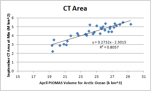
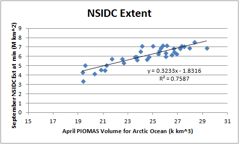
For the above two scatter plots I have calculated April monthly average PIOMAS volume for the Arctic Ocean (including CAA). This has been related to September daily minimum for the two indices stated. The assumption being that April volume within the Arctic Ocean is a significant factor in determining extent/area at minimum.

The R2 when using Arctic Ocean volume is maginally better than that for the whole PIOMAS domain (0.7455) and significantly better than either the peripheral seas of the Arctic Ocean (Arctic Ocean minus Central Arctic) (0.6529) or the Central Arctic region (0.6603) - R2s given for NSIDC Extent only.

Four equations are derived from similar scatter plots, regions being Arctic Ocean, Central Arctic, Peripheral, and Whole PIOMAS Domain. These are applied to the April volumes for each of the four regions for each year for which past data is available 1979 to 2013. While the predictions made depend on their respective April volume region, the predictions are for area/extent in the whole Arctic as covered by NSIDC Extent and CT Area. The residuals of these hindcasts are calculated for each region, these are graphed below for the NSIDC Extent hindcasts and the CT Area hindcasts.





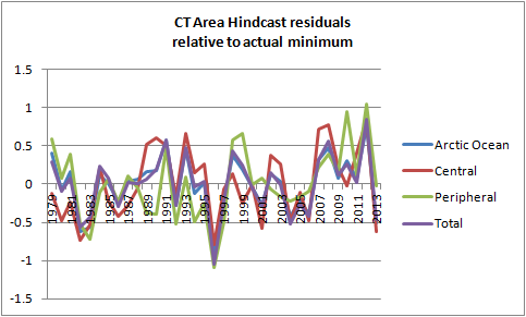
Note that a positive residual represents an overshoot where the prediction exceeds the actual extent/area for the stated year.

It is clear that since 2007 the method consistently overshoots, so a largely one sided set of upper and lower bounds is applied to the prediction for 2014. The upper and lower bounds being simply the greatest positive and negative residuals in the period 2007 to 2012. 2013 is rejected as a weather driven outlier not anticipated to repeat in 2014.


The following table details predictions using the four datasets, the four sets are included for completeness, only the Arctic Ocean prediction is considered worth pursuing at present.



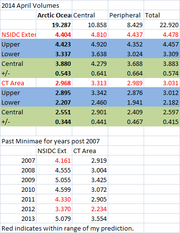
At the top of the table are listed April 2014 volumes from PIOMAS gridded data. In red are the NSIDC Extent and CT Area predictions for each April volume region, however as stated above the predictions apply to the whole Arctic for September daily minimum.

In blue shaded area are shown the upper and lower bounds of the predictions. In green shaded area the prediction is given in terms of a central and +/- symmetrical bounds.

Below the main table is listed the actual minimae in terms of CT Area and NSIDC Extent, figures highlighted in red are within the bounds for the prediction based on Arctic Ocean volume for 2014.

I am not yet making a formal prediction, had I been doing so I would be posting this at my blog (no offense but it would be the right place to do it). However, what can be considered my initial prediction based on April data is as follows:

NSIDC Extent September daily minimum between 4.4M and 3.3M km^2, with the likelihood towards the higher end.

CT Area September daily minimum between 2.9M and 2.2M km^2, with the likelihood towards the higher end.

Next task is to examine the residuals in terms of SLP, Greenland Blocking Index, what else? The aim being to see if the prediction can reasonably be tightened.

[ChrisReynolds]

Just a quick post before I wind down for the evening.

Attached you'll find Greenland geopotential height for June/July/August plotted against snow extent anomaly over Eurasia - taken me ages to find that spreadsheet.

Anyway the correlation between the residuals found above for hindcasts using April Arctic Ocean sea ice volume and the Greenland geopotential height (adjusted for overall increase of atmospheric height) is 0.502. And the relationship between those two sets of numbers has an R2 of 0.2524, being

NSIDC Extent residual = 0.0095*Greenland GPH adj anom + 0.0218.

Not great, but it may help to whittle away some of the bounds on the above hindcasts/prediction. What is interesting is that the attached graphic suggests the Greenland GPH anomaly may be predictable. Unfortunately I last did the work on that in 2012 so don't know about last year...

Anyway, it looks like, for recent years, a good predictor of unadjusted Greenland GPH during the summer is May Eurasian Snow cover. May snow cover depends on April cover in part.

And this April is a record low for Eurasian snow cover.
http://climate.rutgers.edu/snowcover/table_rankings.php?ui_set=1
48th lowest out of 48!

[ktonine]

Chris - I can readily come up with reasons the peripheral and central Arctic lead to lesser correlations.  Have you played around at all with correlations by thickness bins to see if any of them give even better results.  I.e., if we look only at volume of ice with April thickness greater than 2.5m and compare that to September minimum we get and R2 of x.xx?

Note - just asking if you have, not requesting you do so

[OSweetMrMath]

Iceman,

Sure, there are lots of reasons on the forum why things are different, but relatively few mathematical models. This gets at something I was hinting at in my previous post. Most people on this forum are approaching sea ice from a physical model perspective, and are focusing on questions of air temperature, ocean currents, differences in properties of first year vs. multi year ice, etc.

I'm deliberately coming at this from a purely statistical perspective. If all you have is the monthly average ice volume, what can you say about the ice? Granted, we know already that it's declining, and the decline is probably accelerating. That's why it's interesting data in the first place. And it's obviously going to have a yearly cycle. So that constitutes the physical model I'm using. After that, any conclusions I draw have to come directly from the data.

This isn't to say that physical models aren't good or interesting or they can't perform better than statistical models. I'm just choosing to focus on the statistical approach.

crandles,

Those were the posts I was thinking of. Tamino's approach is to use a 5th order Fourier series. The more I think about it, the more questions I have about exactly how to do this. I suppose the solution is to just start trying things. Now I'm curious about whether a wavelets approach would work. I'll have to think about that.

I would guess that for the last 2.5 years (and any future values), he continued to use the values at the last data point where the entire 5 year window is available. A chronic problem of statistical models is that they are better at modeling the interior of data than the boundaries. Just thinking out loud, I wonder if it's possible to extend the data by modeling it as a missing data problem.

[ChrisReynolds]

Chris - I can readily come up with reasons the peripheral and central Arctic lead to lesser correlations.  Have you played around at all with correlations by thickness bins to see if any of them give even better results.  I.e., if we look only at volume of ice with April thickness greater than 2.5m and compare that to September minimum we get and R2 of x.xx?

Note - just asking if you have, not requesting you do so

Kevin,

You'll find attached NSIDC Extent based scatter plots for ice volumes from grid cells above and below 2.25m thick. All for the Arctic Ocean, in no case does R2 exceed the comparable R2 for volume of all categories of thickness. I've done parallel calculations for the peripheral seas (Arctic ocean minus Central Arctic) - as with the case of volume for all categories the R2 in that case is lower than for the whole Arctic Ocean.

Similar to the idea of trying to break things down, a couple of years ago I tried using the distribution of thickness with percentage open water formation to act as a predictor, using individual years %OW profiles applied to a given year's initial thickness distribution in April. The following grpahic is the %OW as a function of intial (April) thickness by decade.



IIRC I found that to be rather clumsy but don't recall comparison with other methods. Maybe I ought to dig out that spreadsheet again...

[Steven]

I last did the work on that in 2012 so don't know about last year...

Anyway, it looks like, for recent years, a good predictor of unadjusted Greenland GPH during the summer is May Eurasian Snow cover.

Chris, the Eurasian snow cover in May 2013 was the lowest on record, so the May 2013 Eurasian snow cover was not a good predictor of the Greenland GPH anomaly in June-August.  But there are probably many other factors related to this that I'm unaware of...

[ChrisReynolds]

Thanks Steven, I'd just not had the time to check.

So I'm back to pondering one of two things on the issue of 2013 - an external random factor acting against snow as a driver (FWIW, Overland Wang and Francis pointed towards May snow as a factor in the post 2007 Arctic Dipole occurrences. Or the early retreat of sea ice off the Siberian coast in years post 2007.

[ChrisReynolds]

I've played around with using PIOMAS gridded data on a per-grid box basis to make predictions but have found it unsatisfactory due to changes in melt behaviour in recent years and the uniqueness of each melt season.

Here's what I've just done, which is simpler approach but shows the same problems.

I've calulated, for each PIOMAS grid cell, the thinning between April and September for each year from 2007 to 2012. This has been used as a set of scenarios, S2007 to S2012. The thinning scenarios have then been applied to all years from 2007 to 2013 on a per grid box basis using the April thickness for each year. The following table of results has been generated. All figures are for PIOMAS volume in September, 1000 km^3.



Along the top is the list of scenarios, so each downward column is the relevant scenario applied to each year (years going across). For example under the S2010 column is listed the September volumes when the thinning for each grid box is applied to the April thickness for each year from 2007 to 2014. The figures in the white central part of the table can be considered hindcasts of September volume, highlighted in Green along the bottom are the predictions using this method for 2014 minimum volume.

In the rightmost pink column are listed the actual September volumes. These are taken from the data provided at my blog, that they agree with the volumes calculated for each year given the year's thinning profile (diagonal figures in bold) is a check that the method works.

Within the central white portion of the table the hindcasts that are above the actual value for the year are in red, those that are below are in blue. Note that S2008/2007 at 6.052 should be blue, not red!

The evident spread of hindcasts makes this method a poor predictor. Note the shift to higher rates of thinning post 2010 as seen by the shift to blue moving from S2007 to S2012. Note that while all years overshoot when using 2007's thinning as a scenario, the opposite is true of 2012's thinnning scenario. 2013 produces undershoots of prediction in every scenario but 2007.

If I had to use this to predict 2014 I'd pick S2010, S2011 and S2012 as the likely forecasts. But i won't be using this method.

[Steven]

So I'm back to pondering one of two things on the issue of 2013 - an external random factor acting against snow as a driver (FWIW, Overland Wang and Francis pointed towards May snow as a factor in the post 2007 Arctic Dipole occurrences. Or the early retreat of sea ice off the Siberian coast in years post 2007.

Thanks Chris.  Which paper by Overland et al. are you referring to?  Do they propose a physical mechanism by which an earlier retreat of land snow cover in May increases the chances of an Arctic dipole during summer? 
(Perhaps it is this paper by Overland et al., pdf, but from my cursory reading that paper seems to mention only the North American snow cover.)

[crandles]

I have thought about trying to pull out data for:

Volume in cells that always melt out (12 of 12 prior years)
Volume in cells that 75% of time melt out (9 of 12 prior years) and volume reduction in those cells
Volume in cells that 50% of time melt out (6 of 12 prior years) and volume reduction in those cells
Volume in cells that 25% of time melt out (3 of 12 prior years) and volume reduction in those cells
Volume in cells that never melt out (0 of 12 prior years) and volume reduction in those cells

I am still trying to figure out if there are any calculations that can be done with such data to get a good correlation with melt volume. Trouble is that low volume in cells that always melt out should mean higher volume melt in nearby cells that don't always melt out but it is to some extent counteracted by the low volume in those cells. Perhaps I would have to try to get a good correlation with actual volume reduction in cells other than the ones that always melt out.

Maybe I will get around to trying it sometime.

[ChrisReynolds]

Steven,

Sorry, yes it is that Overland paper. The paper discusses northern hemisphere snow cover, but mentions north american in particular. What I may be remembering is the contents of an email exchange with Dr Francis. I can't recall if it was myself or her that raised the issue of Siberian snow cover retreat. It was connected with anomalous wave activity found by Hanna in "The influence of North Atlantic atmospheric and oceanic forcing effects on 1900–2010 Greenland summer climate and ice melt/runoff" http://onlinelibrary.wiley.com/doi/10.1002/joc.3475/abstract

I've looked at such wave activity in 500mb geopotential height and suspect it's possible that steering around the Alaskan Rockies is a factor. Looking at contours in 500mb GPH at 63.75degN latitude (attached below) shows that the post 2007 period seems to have a phase delay before the Rockies (by the Gulf of Alaska), with a general rise in the atmosphere after 2007. I suspect that there may be a connection between Siberia and the Greenland ridge in this manner - but frankly such atmospheric science is well beyond me.

Crandles,
I'll have a think about it tomorrow, but it's a fairly complicated coding task.

[OSweetMrMath]

The PIOMAS May data is out. I assume the usual updates will appear shortly, but I want to update my prediction for the September minimum here. The monthly average for May was 21.901 thousand cubic km. This compares to my predicted value of 21.7 thousand cubic km. Since the actual value is above my predicted value, all of my predicted values have been updated to be slightly greater.

In particular, the predicted value for September is now 5.0 thousand cubic km, with 95% confidence interval of 3.5-6.5 thousand cubic km. This compares to my previous prediction for September of 4.7 thousand cubic km, with 95% confidence interval of 3.0-6.3 thousand cubic km.

The attached graph shows the actual monthly ice volume through May (in black) with the prediction based on the April data in red and the prediction based on the May data in orange. The discontinuity between the black line and the red line is this month's prediction error.

[OSweetMrMath]

I have again updated my predictions based on the June data. The predicted value for June was 17.4 thousand cubic km. The actual value is 17.668 thousand cubic km. Once again, this increases my predicted values for all future months, so my prediction for September is now 5.4 thousand cubic km, with 95% CI of 4.1-6.7 thousand cubic km. This compares to my predictions based on the April data of 4.7 thousand cubic km and based on the May data of 5.0 thousand cubic km.