The Slow Transition

[ChrisReynolds]

Cesium,

I'm not sure the idea of weather being uncorrelated at region level is really sound. There might be an argument for two sets of random numbers, a whole Arctic (correlated) element plus a regional dither might be more realistic.

I was thinking if winds are from the South somewhere then there are other places where winds are from the North. However I am not sure what weather conditions you are building in, if you are just doing levels of sunshine and counting on winds in different areas effectively cancelling then uncorrelated may be reasonably OK. It is then the frequencies of the sunshine levels that needs to be realistic - getting two different years to be as far apart as they usually are might be difficult?

Chris:  It's interesting to think about how to build that intermediate model.

Crandles:  For this model, the assumption is that "weather", of whatever kind, is constant random noise.  (And evenly distributed within the min/max given by historical data since 1978.  e.g. There are no 100 year events other than those recently seen.)

Actually I was pondering it more today. You will probably get net warm and net cool seasons, different modes (AO/PNA/ENSO) will impose their own patterns of variability in temperature. But on balance, even in a warm or a cool year you can get substantial regional differences. So I no longer think it is such a strong objection - uncorrelated is probably OK simply to impose some stochastic variation from which the monte carlo will draw a probability distribution.

I won't get round to it tonight, but I am going to start a new thread. I've been playing around with the following equation.

dh/dt = 2592 * k (to - ts) / hpl.

2592 = timescale adjustment for monthly calculation.
k = thermal conductivity of ice
to = temperature at the ice/ocean interface
ts = surface temperature
h = ice thickness
p (rho) = density of ice
l = latent heat of fusion

It's not very good, it 'doesn't get' late open water and very low ice thicknesses - they cause overshoots. It has no snow, so it often overshoots. No ice motion, it's just a column of ice. And I'm using NCEP/NCAR monthly data and PIOMAS monthly data, I have used synthetic winter temperature profiles for a daily run over winter, but by April there are large errors in many years, some of which seem to be accountable through ice movement, late refreeze, etc.

Anyway, here is one of the more flattering plots  . April thickness for the ESS from PIOMAS, and April thickness for a 1mX1m ice column subjected to the monthly average NCEP/NCAR temperatures for the ESS. EDIT - that's April thickness, the simple model of growth is seeded with September thckness.

Decided to add another which should be self-explanatory.

[SATire]

When y < 1, the function is a sigmoid, so considerably less nasty.

Congratulation - you made it. The nasty part is to get from that solution in x(y) form to a more suitable y(x) from... Beautiful for curve fitting is something else, but numerically that is no problem, of course.

Please have fun with integrating differential equations with wolfram alpha. Some years back that work was really blood and tears...

[OSweetMrMath]

What do you think is going on here? You are seriously underestimating my mathematical background, and being patronizing about it on top of that. Yes, I know how differential equations work. Yes, I can use Wolfram Alpha to find numerical solutions. Turns out I can just as easily write my own numerical solutions. Your attempts to educate me on how math works and on "math language" are not appreciated.

[SATire]

Chris, maybe the link to wolfram alpha provided above is more usefull for you than for other poeple:

That wolfram alpha is very good in obtaining analytical solutions of differential equations, wich are very hard work to solve "by hand". So if you want to integrate an model to get a function you want to fit to data that tool could sometimes be helpful for you. But sometimes that form may be nasty and not so helpful as in that example given in the link above.

If you want to fit numerically you may also ignore this idea, since in that case you may solve the differential equation numerically using standard methodes, too.


To everybody reading here:
I am sorry if I educate poeple to much. That is the usual behaviour of a physicist and that is usually not appreciated - that's life.

[OSweetMrMath]

Let's leave aside the fact that most of your attempts to educate me have not been correct. In my experience as an educator, "students" are more receptive when you don't talk down to them and don't make assumptions about their lack of knowledge of a subject.

Further, I don't participate on this forum to be educated. I participate to have a conversation. Learning things along the way is a natural part of this, but not why I'm here. I assume this is true for most people here. In particular, I don't always agree with Chris, but I have a ton of respect for all the work he does, and I would never presume to educate him.

Also, I'm amazed by your shift in attention from me to Chris. Very striking.

[SATire]

OSweetMrMath,

I am here to be educated. Nearly everything I know about sea ice I did learn here. So I want to give back a bit by explaining some things from the field where I am an expert in. Surely I am not the only expert in my field - so please feel free to ignore my posts if they do not help you. I have the hope my post may be of help for someone else and as long as poeple ask me I will answer.

So please - if you found some error in my post, please say that. I am in no way error-proof and already quite rusty e.g. in integrating. 

[ChrisReynolds]

SATire, OMrSweetMath,

Thanks for the interesting discussion, although a lot of it went over my head I got the generalities in the way that one can get a complex argument at the time, but an hour later it is gone. I am in no way fit to adjudicate.

Thanks for the tip regards WolframAlpha. I used to use Wolfram Mathworld when I was messing around with digital signal processing as a hobby. As an indicator of my innate mathematical ability, it once took me a week of work to understand the Fourier Transform decimation in time algorithm - In maths I am a plodder.

[ChrisReynolds]

A simple thermodynamic model of sea ice growth is

k(To-Ts) / h = p l dh/dt

In plain english...

The heat flux though a sheet of ice over water is determined by the temperature difference through the sheet of ice and the ice thickness (h). The temperature difference across the ice (To - Ts), which is the difference between the surface temperature (Ts) and the temperature at the ice/ocean boundary (To). EDIT - forgot a crucial detail - To, the temperature where ice and ocean meet at the underside of the ice is set to -1.8degC.

That's the k(To-Ts) / h bit, where k is the thermal conductivity of ice ~2.2W/m degC.

Now assume that all this heat flux goes into making ice at the ice/ocean boundary. A complication here is heat flux from the ocean, e.g. due to AGW, if needed this can be deducted from the heat flux through ice to reduce the amount of heat flux that makes new ice at the ice/ocean boundary (underside of the ice). But keep it simple, also keep it simple by neglecting snow.

Here we need to convert our heat flux into a measure of joules (energy) per cubic metre of ice.

The latent heat of fusion is the energy that water gives out as it turns into ice, that's l ~ 333.4kj/kg.

The density of sea ice is about 917kg/cubic metre (m^3).

kj/kg * kg/m^3 = kj / m^3. That's our conversion from energy into volume of ice.

That's the p l dh/dt bit. In plain english that is; for each incremental interval of time multiply the latent heat of fusion by the density of ice to get the energy during that interval, as the units are in seconds the time interval is in seconds.

So if you want to have a change in ice thickness equation you just rearrange the first equation to give:

k(To-Ts) / h p l = dh/dt

This physical equation is the basis of the growth/thickness feedback.

[crandles]

This physical equation is the basis of the growth/thickness feedback.

I have a slightly different query on that last graph.

If you start with near zero thickness you get near 2.5m of thickening for a total thickness of 2.5m

If you start with near 1m thickness you get near 1.5m of thickening for a total thickness of 2.5m

So far so good, you end up with 2.5m thickness regardless of starting thickness. (Snow would reduce that 2.5m to a lower thickness if snow was being built in.)

But if we started with 2.5m thickness, should we expect any thickening at all? I would expect no, but the last graph seems to suggest you still get substantial thickening.

Why does the graph tend to level off rather than carrying on steeply down after 1m initial thickness and head towards initial thickness of 2.5m resulting in zero thickening?


Sorry, think I was being thick.
I was assuming a constant upward heat flux resulting in a steady end of winter thickness almost regardless of initial thickness whereas you seem to be doing something different:

specifying a constant (To - Ts) differential? or specifying To and providing a set of Ts s' over the course of an Autumn & Winter? or ...

[cesium62]

Decided to add another which should be self-explanatory.

Cool.  So we understand winter thickening fairly well.  If we can make good guesses about future values of Ts and To from year to year, we can probably reasonably well model winter thickening?  (Can we quantify what ... percentage ... of winter thickening is explained by the heat flow model?)

Does Ts and To also tell us anything about summer melting?  Do things like albedo, weather, and wind swamp the changes that this simple heat-flow model suggests would occur?  Or does this heat flow model explain a big chunk of summer melting?

[ChrisReynolds]

Cesium,

Sorry I forgot to add in the post above that To, the temperature of the ice/ocean interface at the base of the ice is -1.8degC, which is the typical freezing point of sea water. Because the lower temperature is set things like ocean heat flux from ocean warming needs to be treated as a flux of energy that is deducted from the flux through the ice. Semtner 1975 specify this flux as 1.5kal/cm year.

If we can make good guesses about future values of Ts and To from year to year, we can probably reasonably well model winter thickening?  (Can we quantify what ... percentage ... of winter thickening is explained by the heat flow model?)

To make the two graphs shown above I've used data for the ESS. The area of the ESS is such that it is relatively easy to get NCEP/NCAR to make timeseries of monthly temperature, then I have PIOMAS gridded thickness for the ESS to compare to.  But I have not accessed the PIOMAS gridded snow product, I'm going to continue to neglect snow.

Neglecting snow might seem like a big problem, it is for comparison to reality or to a more advanced model like PIOMAS. However the simple model here is really only answering the question - what does the thermodynamic growth of ice look like for a column of sea ice subjected to the average temperure of the ESS from September to May. Note that by May volume sometimes starts dropping - there is no sun and no provision for melt in this model.

Can it be used to try to ascertain real world thermodynamic growth for comparison with PIOMAS? Well the errors are rather large.



What happened in 1989? That will become clear shortly.

Anyway here are a selection of years thickening profiles for the ESS from PIOMAS and the simple model. Actually my spreadsheet is called 'column model', which is probably a better term. Note that a year is for Jan to April, with the preceding Sept to Dec being included in the next year. i.e. Sept 2006 to April 2007 is listed as the year 2007.

1980


1989


2000


2010

2010 ends with PIOMAS higher - is this due to th export of thick MYI from the Central Arctic reaching the ESS about that time?

2012


2014


So the model does rather a poor job when compared to a far more sophisticated model, however this is to be expected given the model's simplicity and the lack of factors such as snow, ocean heat flux, and sea ice movement.

Looking at regional volume data for the ESS, the following is a plot of volume from grid boxes above and below 2m thick in January, on the basis that ice over 2m thick by January is likely to be multi-year ice. First year ice doesn't generally thicken to over 2m thick by January.



The 1989/1990 switch in errors between the model and PIOMAS is seen to happen as the ESS switches abruptly from thicker to thinner ice (implying a MYI to FYI switch). Thinner FYI will show stronger thermodynamic growth, so after 1990 the simple model regularly overshoots PIOMAS.

So what does a scatter plot of PIOMAS and the simple model look like after 1990, when the pack is mainly first year ice.



The result could be thought to imply that as PIOMAS declines substantially (horizontal axis), the simple model (vertical axis) hardly declines at all, which would reject the simple model as being of any use. But before I stop here, I'll show the simple model and PIOMAS timeseries for 1990 to 2014.



Here it is clear that the large variation in the horizontal axis of the scatter plot is the interannual noise of the PIOMAS data (it's a far more complex model with more factors). However the trends in decline for the two models are similar, albeit that the PIOMAS uncertainty of trend will be far broader than for the simple model.

So, despite the problems caused by the model's simplicity, I think it is worth looking at how it behaves with variation of parameters such as initial thickness and winter temperature.

[Steven]

I've been playing around with the following equation.

dh/dt = 2592 * k (To - Ts) / hpl.

2592 = timescale adjustment for monthly calculation.
k = thermal conductivity of ice
To = temperature at the ice/ocean interface
Ts = surface temperature
h = ice thickness
p (rho) = density of ice
l = latent heat of fusion

...  To = -1.8 degC
...  k ~ 2.2W/m degC.
...  l ~ 333.4kj/kg.
...  p ~ 917kg/cubic metre (m^3).

Chris, this differential equation can be solved in closed-form, e.g. using separation of variables.

If the sea ice at a given location and date has a certain thickness (say, c meters), then the thickness n days later is

sqrt( c² + n(To-T)/804.2 )

where T is the average surface temperature during these n days, in degrees Celsius, and To = -1.8.

E.g., if the ice thickness at the beginning of October is zero, and the average surface temperature from October 1 to April 30 is -20°C, then the ice reaches a thickness of 2.19 meters at the end of April, according to this equation (c=0, n=212, T=-20).  If the ice was already 1 meter thick at the beginning of October (c=1) then it reaches 2.41 meters thickness at the end of April, etc.

Of course, as you say, this equation doesn't include "factors such as snow, ocean heat flux, and sea ice movement".

[ChrisReynolds]

Thanks Steven,

You must have been reading my mind.

I've been working off an old 1975 paper (Semtner).
http://journals.ametsoc.org/doi/pdf/10.1175/1520-0485(1976)006%3C0379%3AAMFTTG%3E2.0.CO%3B2
Scroll down and at the end the Appendix is for an even simpler model, those two words 'even + simpler' caught my attention. It's that which I've been using, but much in the rest of the Semtner paper is at the core of most (all?) of the papers I've read describing sea ice models.

But there's the same equations here:
http://www.unis.no/48_HSE/Info%20Lessons/Sea_Ice/Introduction%20to%20Sea%20Ice.pdf
Anyway on page 8 of that there is an equation for thickness of ice as a function of freezing degree days. The FDD definition I get. But when I try to evaluate that equation on page 8 it comes out wrong, and I haven't been able to figure out how to get there using the differential equation I posted - my calculus is really rusty.

But what you've just posted looks like what I've been trying to work out.

Tomorrow I'm going to be a mixture of really busy or recovering from what looks like a rather involved wisdom tooth removal, but will have a proper look on Wednesday, got the day off to put my feet up.

Thanks.

EDIT, the next day.

I've found the error in my spreadsheet that was puzzling me. I'll post in the next few days. Now the Freeze degree days calculation compares well with my calculation of ice growth by month (slight difference as the per month calculation used 30 day months simplification). I'll follow up over the weekend.

[ChrisReynolds]

Rather delayed due to work, but I'll continue.

Steven has helped me understand how thickening as a function of freezing degree days (FDD), as a result I can see where I went wrong in evaluating the equation I already had. But before I go onto that I'll go over some results from evaluating the simple model on a daily basis.

I only have monthly average NCEP/NCAR temperature for the East Siberian Sea (ESS), I wanted daily, but haven't got round to coding to access the daily data files. So I have created synthetic daily temperature data by fitting a quadratic to September to May temperatures.

A quadratic equation is of the form:

y = ax^2 + bx + c.

So for each year I calculate a, b, and c. For example for 2014 the monthly average temperatures in blue create a quadratic fit in black, with the equation as shown on the graph below. Note that for each year, the stated year is for 15 September of the previous year through to 15 May of the stated year, e.g. 2014 is 15 September 2013 to 15 May 2014.



A start thickness of 0.1m is used, because the equation k(To-Ts) / h = p l dh/dt has a denominator of zero using thinner initial ice creates unfeasibly massive heat flux and massive subsequent ice growth, using zero thickness creates a division by zero error. The synthetic daily temperature profile is set such that temperature above -1.8degC is set to -1.8degC. Because the ice/ocean boundary temperature is set to -1.8 this creates a condition of no ice growth until temperature drops below zero.

Below I have plotted the synthetic temperature profiles and plotted thickness and heat flux through the ice for three example years.

2014





2007





2000





Daily ice thickness gain is directly proportional to the above shown heat fluxes (so the curve looks identical in form), the constant of proportionality is 0.000259.

To get a feel for what is going on in the above graphs I've applied a steady -10degC surface temperature from 24 Sept through the winter.



Here as soon as the temperature difference is applied heat flux (and ice growth) jumps up, then the insulation of thickening ice takes over and the heat flux drops, allowing a more gradual slowing of thickening through the winter.

In reality there is no immediate step to colder temperatures, the gradual setting of the sun is causes a gradual cooling, which is then augmented as the polar night spreads south (reducing heat transport from nearby regions to the south). And in reality as the sun sets the process of heat loss from the ocean increases until the surface hits freezing point (about -1.8degC), but even then there will be heat flux from lower ocean levels which is not incorporated into the model.

This makes the three years heat flux and thickening a combination of gradually decreasing temperatures, together with the increasing insulation of thickening ice. Hence the more rounded profiles of the three years as opposed to the initial spike in heat flux shown in the constant -10degC.

Now it is worth looking at the effect of initial (September) thickness.



In the above ideal case the synthetic 2012 winter temperature profile (Sept 2011 to May 2012) is used. A simple relationship is seen, with thicker ice thickening less over the winter than for the case of no ice (initial thickness 0.1m). Using PIOMAS data to seed the September initial thickness, and the NCEP/NCAR monthly temperatures for each winter adds noise to the relationship.



PIOMAS thickening is shown on the above graph, this adds further noise because unlike the simple model PIOMAS has ice transport, mechananical deformation, snow, and ocean heat flux.

I've calculated the effect of delaying the start of the freeze, here by applying a continuous -15degC surface temperature from a certain date.



Looking at the end thickness on 15 May and the proportion of the freeze season, the impact of delayed freeze can be seen. For 1 October being 100% of the freeze season, and for the 1 October case thickness on 15 May being 100% thickness:

For 87% of the freeze season growth is 93%.
For 74% of the freeze season growth is 87%.
For 61% of the freeze season growth is 79%.

So because of the early rapid growth rate shortening the freeze season does not impact the end season thickness to the same degree as growth season is shortened. For a halving of the freeze season, end season thickness only drops by around a quarter.

So under relatively realistic conditions the simple model of ice growth produces an ice thickness of around 2m thick for near ice free initial state in September. Thicker ice grows less vigorously. But because most of the growth happens early in the freeze season, a delay to start of freeze does not have as much of an effect on thickening as one might suppose.

To get a feel for how much further thinning may occur in winter rather than look at a daily or monthly calculation it is best to switch to the Freezing Degree Days perspective. I aim to post on that this week.

[Tor Bejnar]

You've been doing awesome work, Chris.  (And I'm glad there are folks able to check your work, too.)  Your work (often, when it's not too over my head) helps me to better understand what is happening.

[sofouuk]

it's not just the quality of the work, but the clarity with which it's presented, that makes it so valuable

[ChrisReynolds]

Tor, Sofouuk,

Thanks for that. I had been wondering if what I was doing was anymore than me following something that interested me. I'm happy with that, but if it's only interesting me then I should keep it to myself. If others find it interesting/useful then it's been worth posting.

I'm glad there are others around who will tell me when I've screwed up. I don't feel I am beyond that on the above comment.

[ChrisReynolds]

If it is not already apparent, by the end of this comment it should be clear why I have put these comments in this thread and not started a thread for them alone.

The Polar Science Centre has a useful page on Freeze Degree Days in the Arctic:
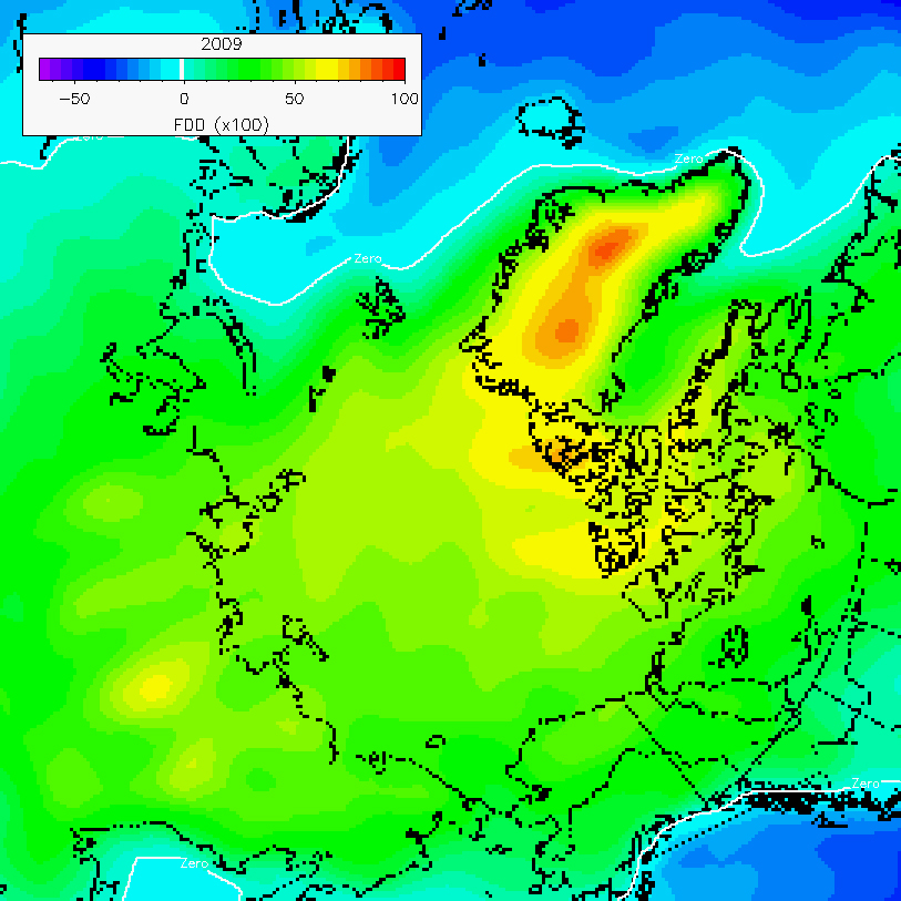
http://psc.apl.washington.edu/nonwp_projects/landfast_ice/freezing.php

From that here are the FDDs worked out for the Arctic over winter 2009 (1 September 2009 to 31 May 2010).



I'll be sticking to the alternate convention used in my comment above, that the winter of a particular year is from the previous September to the April of that year. But it's worth keeping in mind the sort of FDDs for 2009 and as an example the FDDs calculated for 1949 as shown below.



FDDs are very simple to work out. Freeze degree days is the sum of; the number of days below zero degC multiplied by the temperature for each day. As I have monthly average data for temperature I'll be working on a monthly basis, so for example:

December average surface temperature over the ESS in 1979 was -32.069degC, over 31 days that is 994.14 days degC (not days per degC, but days degC), calculate the FDD for each month and sum for the period September to April gives the FDD for the winter. However as I'm working off a baseline of freezing point for sea water I have added 1.8degC to get the difference between -1.8degC and the surface temperature in each month - that's what will go into an equation.

Steven was good enough to work out the equation I needed, although I already had it and was doubting it was right - that turned out to be because of a basic error in my spreadsheet. Anyway the equation was

Thickness at day n = sqrt(InitialThickness^2 + n(To-T)/804.2 )
(sqrt is 'square root', and '^' means 'to the power', i.e. InitialThickness squared.

Rewriting this in terms of FDD over September to April gives:

Thickness at day n = sqrt(InitialThickness^2 + FDD/804.2 )

Where my calculation of FDD is as explained above.

Thats the maths done with, from now on we can just think of FDDs as a handy way of combining changes in temperature and changes in freeze season length (i.e. the overall intensity of cold through the freeze season) to look at the effect on simple thermodynamic growth of sea ice.

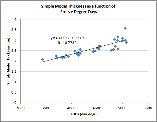
The following graph shows April thickness from the simple model calculated as a function of each year's FDDs over winter, with September initial thickness being from the PIOMAS model.



And for comparison here is PIOMAS April thickness as a function of each year's FDDs.



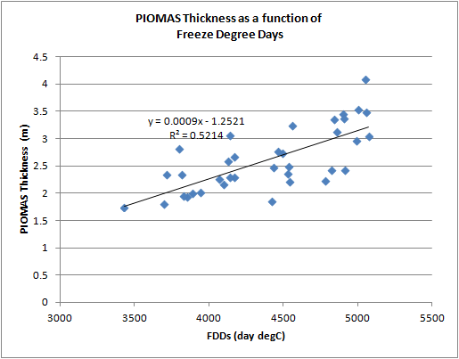
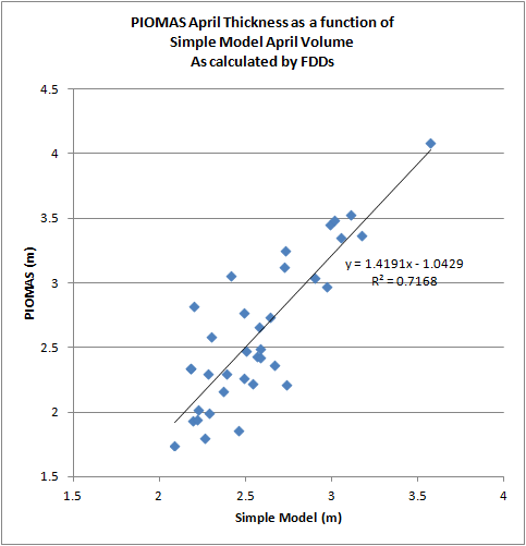
The PIOMAS relationship is weaker (R2 of 0.52) than the simple model (R2 of 0.77). As I will show below over this period the simple model is approximately linear, so without the complication of PIOMAS September thickness being used we'd probably expect that the simple model R2 for a linear line of fit should be close to 1. PIOMAS is of course a weaker fit (more scattered points) because there is a lot more going on in that model an it is closer to reality. Yes the simple model of ice growth is a bit crap, but it isn't totally useless. The scatter plot of PIOMAS and simple model April thickness shows a clear relationship, and at an R2 of 0.72 the simple model explains a significant amount of the variation in PIOMAS. PIOMAS holds a far more general form, but during winter PIOMAS thermodynamic ice growth is dominated by the simple model's physics.



If we set the simple model's initial thickness to zero then we can get a feel for how FDDs relate to April thickness in the simple model.



This graph is basically a square root plot, because taking an initial thickness of zero the equation becomes.

Thickness at day n = sqrt(FDD/804.2082)

As the 804.2082 part doesn't change it plays no role in the evolution of the graph, except by constantly scaling FDD.

But I have plotted the above with thicknesses above 1.5m highlighted by blue dots and their own trend. Down to a thickness of around 1.5m and an FDD of around 2000, April ice thickness declines linearly in relationship to FDD.

I'm interested in 1.5m as a rough figure of the sort of winter thickness that could bring about a virtually sea ice free state. I hope that those expecting a rapid transition find that this is not too conservative.

Ed Blanchard Wigglesworth gave some interesting results from PIOMAS (hat tip to Crandles), around 55 minutes into this Youtube video:

That should start where you need.

This is the graphic I'm interested in.



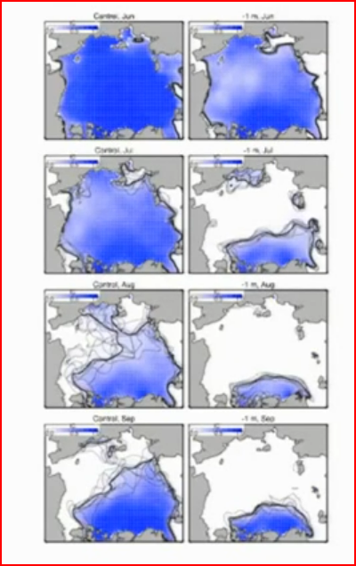
What the PIOMAS team did was artificially thin the sea ice by 1m in May (I think). Then the model was run using a selection of weather from recent years. The modelled ice collapses with an extraordinarily aggressive spring melt to give only remnant of thick ice off the northern coast of Canada and Greenland. In the graphic below 'control' is a set of typical PIOMAS runs for recent years (left column), 'experiment' (right column) shows what happens when the ice is thinned by 1m. Rows go from May to September.

Typical thicknesses are around 2m in recent Aprils, so somewhere between 2m and 1m thick there is potential for extremely aggressive loss of ice and virtually ice free conditions. Let's say that an April thickness of 1.5m is a reasonable compromise position for the start of the sort of losses seen in the '1m experiment'. How far away is 1.5m April thckness in terms of FDD? Well, it's an FDD of around 2000.

As shown in the graphic at the start of this comment FDDs for September to May are typically higher for a recent year like 2009. I have also calculated FDDs for the post 1979 years and plotted in the following graph.



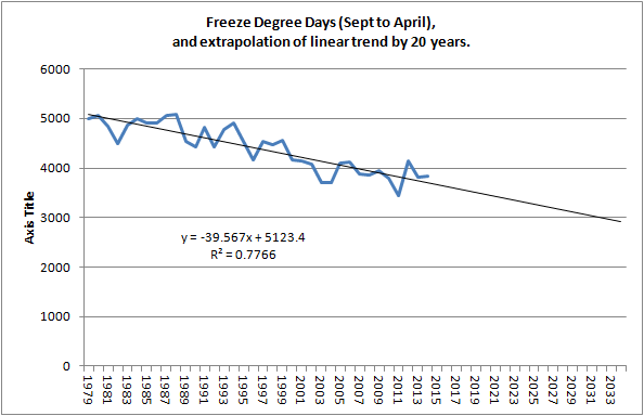
The extrapolation isn't meant to be a prediction, it's just a graphic tool to show that for FDDs to drop to around 2000 there has to be a substantial winter warming and/or a shortening of the freeze season.

Now, all of the above has been worked out using data for the East Siberian Sea (ESS), which has been seasonally ice free for some years, along with the other peripheral seas. The question has never been when will those seas beceome virtually ice free in most summers, since 2007 that has largely been the case in most years. The question is when will the Central Arctic become virtually seasonally ice free, 2012 showed that for that to happen very early melt of the peripheral seas is needed to allow substantial losses in the Central Arctic. And as the first graphic of this post shows FDD for the Central Arctic is higher than for the ESS.

Since 2001 average extent of the Central Arctic on 15 April has been 4.45M km^2. In September 2012 this had dropped to 2.81M km^2, a drop to 63% of maximum extent. To get down to 1M km^2 (August extent in the PIOMAS 1m thinning experiment) would be a drop to 22% of mid April extent.

What I hope I have shown is that the freeze season gain of thickness (hence volume) is powerful enough to keep up with summer losses, until the freeze season experiences such a combination of warming and shortening that April thickness drops to well below 2m thick. A reasonable ball park figure for expecting a virtually sea ice free state is something like 1.5m thick, but for a reduction in thermodynamic thinning to cause that 25% reduction in thickness would need a halving of current winter severity as measured by FDD.

[Tor Bejnar]

Thanks, Chris!
I know this is beyond the 'simple model', but what you write gets me to think about what could significantly lessen the intensity of central Arctic Ocean winters beyond the 'slow' slog of increased green house gasses.  My quick brainstorm: 1) deep snow in late September that is blown off (or rained on) in March, so melt ponds can form; 2) winds export so much ice during the winter that the Arctic Basin has mostly thinner 'previously marginal sea' ice.  These, of course, include the 'perfect storm' that 'could melt all the Arctic sea ice in two years.'

[ChrisReynolds]

I think the biggest issue in making Central Arctic winters more mild is heat transport from mid latitudes. The simple model doesn't contain any ocean heat flux, if Atlantic Water were mixed somehow to break down the halocline and allow it to get to the underside of the ice that would be a flux of heat you could effectively subtract from the heat flux that goes into making ice - the result would be thinner ice. The problem for me on that count is that I haven't read anyone make a really convincing case for that happening. However even without that mixing, an increase in warmer Atlantic Ocean influx would lead to more heat flux (though not as great as direct contact) and should thin ice.

Snow looks likely to be a negative feedback. There is a paper that shows that reduced snow thickness is due to less ice at the end of the summer and open water persisting into the autumn. Less snow means thicker ice because there is more heat flux through the ice, snow insulates the ice and reduces thermodynamic thickening. However if there is a large influx of warmer air from mid latitudes then it is possible that this could bring with it more snow. While not implemented in the simple model (it's not that much more work to implement it), increased snow could be seen as a reduction in FDD because you could still consider snow's impact on the temperature at the top of the ice.

Your point 1 is mainly a spring/summer effect, summer melt is more tricky to work out and isn't crucial for the point I was making here. There will be greater volume losses to come in the future during spring/summer, but the PIOMAS experiment outlined above suggests significant thinning is needed for losses to create summer conditions for a virtually sea ice free state.

Your point 2, yes a massive export of ice (in March/April) could push the ice thickness across the basin low without time to recover to full thickness, this could result in a crash greater than 2012. But I am not sure there is a precedent for this, and anyway Tietsche et al suggests that the next winter conditions would start to approach normal with massive loss of heat gained and a reversion to the local equilibrium.

By 'local equilbrium' I mean that the ice long term is not in equilibrium, it is chasing the impact of AGW as it finds a new equilibrium in a changing environment. But 2007's recovery in 2008 shows how after an impact the ice 'tried' to get back to conditions that prevailed before 2007 - those conditions were a local equilibrium in an overall changing state.

[Tor Bejnar]

Your (appropriate) criticism of my #2 (late winter winds blowing thick ice to Iceland, getting replace by thinner marginal-sea ice that doesn't have a chance to thicken) - no know prescident - is about the same for your 'mixed Atlantic waters'.  Although there are not specific prescidents for these, we know the jet stream is behaving odd at times and there are discussions about changing Hadley Cells, and oceanic circulation is changing too. These are the realms that may cause a dramatic change in the central Arctic's current condition.

(My spring rain idea is just to have a mechanism to get rid of the 'lots of snow' that would reflect sunlight and prevent ponding in the spring/summer.  Otherwise, I think the thinner ice under the thick blanket of snow would not have insignificant surface melt.)

[DavidR]

Chris,
This graph is very misleading as it continues for two months after the start of the melt  season. While the volume increase in the central  Arctic may continue well into April little ice that started freezing in December will be in that  region.

I've calculated the effect of delaying the start of the freeze, here by applying a continuous -15degC surface temperature from a certain date.



Looking at the end thickness on 15 May and the proportion of the freeze season, the impact of delayed freeze can be seen. For 1 October being 100% of the freeze season, and for the 1 October case thickness on 15 May being 100% thickness:

For 87% of the freeze season growth is 93%.
For 74% of the freeze season growth is 87%.
For 61% of the freeze season growth is 79%.

In most  years, by 15 May, the area melted out is approximately equivalent to the area of re-freeze after 1 Jan.  So  while it may be feasible for an individual floe to stay in the described state from 1 Jan to  15 May, in practical terms most  of the ice has been in melt for two months by that  time.

At the start of the melt  season approximately  4M km^2 of ice is less than a metre thick. This equates to the refreeze since about the beginning of  December. Little of this ice will get significantly thicker as it exists on the boundaries of the pack.

[crandles]

Thanks Chris for putting this up.

This looks pretty good:



is saying we are at about 3800 FDD.

You are saying we need to get down to 2000FDD to get 1.5m thick ice (which might then melt out) per



and 2000FDD is a lot less than 3800FDD.

My intial reaction was that we are already at maximum average thickness of about 1.7m not the 2.2m that the above graphs suggests. However average thickness is not relevant that is distorted low by large areas of thin ice. To melt back below 1m km^2 we need to melt areas where the thickness is currently getting up to over 2m thick:



This seems to suggest that neither ocean upward heat flux nor snow cover is very significant. Otherwise the ice would actually be quite a bit thinner than the model would suggest? (or is there a fit of data or perhaps 'If we set the simple model's initial thickness to zero' is a significant 'fudge' factor?)

If you have shown that neither ocean upward heat flux nor snow cover is very significant, then this seems a very significant finding to me.

.

Not too sure about 1.5m. I think we are largely melting out areas up to about 1.8m thick in a high melt year. It might have to get thinner than 1.8m in order to melt a longer distance into the ice pack but I don't have much feel for whether this means 1.7m or 1.5m or thinner. I am concerned that the difference between 1.7m and 1.8m might be significant but have little if anything to back that up.

[Comradez]

So, if a strong melt year (like 2012) can melt out ice that is 1.8 meters thick instead of 1.5 meters thick, then what are we looking at for Freezing Degree Days (FDDs) that we need to get down to before we can melt out all of it?  2800 FDDs?  If so, then we are still looking at 2035 before we get there, according to the linear trend.  Maybe there will be an anomalous year before then where both the FDDs during the winter are below trend and the melting season is above trend, but even so, we are looking at 2030 before we can expect a year of complete melt-out. 

[jdallen]

I'd say this line of analysis is heading in the right direction.

I'd not be quite so quick to dismiss the effect of heat in the ocean, or the insulative value of snow on the ice.  It might be useful to consider the degree day value as reflective of "pressure" in the system to export heat.  We actually can make a reasonable estimate of the "volume" of heat exiting via radiation from the upper layers of atmosphere. The tricky bit is evaluating the exchanges across boundaries to reach the upper atmosphere.

[ChrisReynolds]

David R,

The monthly average volume peak for the Central Arctic is in May.  In that region in 2014 peak volume was on 12 May 2014 in 2002 it was on 27 May, mid May is fairly typical for peak volume there. Because most of the thickening is in the early part of the season changing to April wouldn't affect the results much, changing to March would be too early.

Crandles,

Yes we already melt out ~2m thick across the peripheral seas in most summers, but that isn't the issue. Even with a year like 2012 with pack thickness around 2m right into the Central Arctic there just isn't the time in the melt season to make massive inroads into the Central Arctic. The issue is that the rate the ice edge recedes must increase substantially in order for it to recede into most of the Central region in the available time.

PIOMAS shows that when artificially thinned by 1m early in the melt season, the ice edge recedes at what are, from out perspective, unprecedented rates, this allows the ice edge to get right into the Central region very quickly. The point about 2012 is that even with the best conditions and near 2m thickness across most of the pack the drop from maximum winter extent was only around 60%, to get down to 1M km^2 would need a drop of around 20%. While substantial time is taken up melting ice outside the Central Arctic I struggle to see how such a drop is feasible. What can bridge this gap in credibility (as I see it) is a substantial drop in maximum volume.

I certainly wouldn't go so far as to say that any of this shows that snow and ocean heat flux are negligible, that would take a much more advanced accounting of snow depth and pack movement. The errors between the simple model and PIOMAs for the ESS are evenly spread between +ve and -ve, this suggests that ocean heat flux and snow are not the only factors (they should mean PIOMAS is regularly thinner than this simple model).

Here are average thicknesses for April 2011 to 2014 in metres.

Okhotsk, 0.6
Bering, 0.6
Beaufort, 2.3
Chukchi, 2.1
ESS, 2.1
Laptev, 1.6
Kara, 1.2
Barents, 0.7
Greenland ,0.9
Central, 2.4
CAA, 2.0
Baffin, 1.0

Away from the influence of the Pacific and Atlantic, grid box effective thickness within the Arctic Ocean outside the Central Arctic tends to be around 2m.

Comradez,

I agree, but as you say 'according to the linear trend', a linear trend extrapolation is little more reliable than a more complex function. I just wanted to show how far from serious winter thinning we seem to be given past behaviour.

[ChrisReynolds]

I'd say this line of analysis is heading in the right direction.

I'd not be quite so quick to dismiss the effect of heat in the ocean, or the insulative value of snow on the ice.  It might be useful to consider the degree day value as reflective of "pressure" in the system to export heat.  We actually can make a reasonable estimate of the "volume" of heat exiting via radiation from the upper layers of atmosphere. The tricky bit is evaluating the exchanges across boundaries to reach the upper atmosphere.

I don't dismiss those factors, I've just not factored them in preferring the simplest approach, they introduce more variables that can be hard to put a figure on. However with regards snow that is addressed in the appendix to the Semptner paper (see message 162 first link), as well as in the main body of the paper, but I find 'an even simpler model' appealing because I'm carp at maths.

Ocean heat flux is easy to apply, the temperature difference between surface and base of the ice drives a flux of heat (actually energy), an ocean heat flux through the ice does not involve forming ice to the underside of the ice. So the initial equation starts as:

k(To-Ts) / h = p l dh/dt

and becomes:

k(To-Ts) / h = p l dh/dt +Oflux.

Where Oflux is the ocean heat flux. In other words the Oflux term diverts off some of the energy that would otherwise have gone into making new ice.

[jdallen]

Chris - being able to factor in flux from the ocean is a plus.  I agree that sorting ot factors like snow are fiendishly complex. It starts by considering differential thickness of cover and insulative value and only gets worse from there.

I guess what it does identify are some wild cards which provide us with greater uncertainty.

[Steven]

...with regards snow that is addressed in the appendix to the Semtner paper (see message 162 first link), as well as in the main body of the paper

The Semtner paper suggests the thermal conductivity of snow in the Arctic is about 1/6.6 times the thermal conductivity of sea ice, empirically.  So snow is a better insulator than sea ice, by a factor of about 6.6.  (This probably depends on factors such as temperature, salinity etc.)

If the ice thickness (height) is h meters, and the snow depth is hs meters, then the simple model for ice thickening in the appendix to the Semtner paper is:

dh/dt = C (To - Ts) / (h + 6.6 hs).

The factor C is proportional to the ratio of the thermal conductivity and the density of the ice, and is assumed to be constant for simplicity, C ≈ 1 / 1608.4.  Time is expressed in days.

There is probably no closed-form solution to this differential equation.  But of course it can be solved numerically, if surface temperature and snow depth are available (e.g. gridded PIOMAS snow depth?)

[ChrisReynolds]

Thanks Steven,

Yes there is gridded snow data for PIOMAS, and now I check, it is available up to August 2014. It's expressed as snow-water equivalent depth.
http://psc.apl.washington.edu/zhang/IDAO/data_piomas.html

The question is how far do I want to proceed, and at what stage should I do what I have long pondered, try a single column model thermodynamic that works during the melt season too based on the PIOMAS model itself. I've thought about that because I'm interested in the effect of thinning ice on the melt season. I've looked at it, but there are ample places for an amateur like me to trip up.

JDAllen,

Yes there are uncertainties, the aim should always be to reduce them where possible to get a feel for how wide the uncertainties might affect the outcome. With regards ocean heat flux, if you click on the above link you'll see a set of derived data from PIOMAS. One is Oflux (Ocean heat flux used to melt ice, unit: (meter of ice)/s). Unfortunately this only runs to 2004, after which the really interesting stuff happened. I have looked at it, ages ago, but the lack of data after 2004 meant I didn't really spend much time on it.

[crandles]

I certainly wouldn't go so far as to say that any of this shows that snow and ocean heat flux are negligible, that would take a much more advanced accounting of snow depth and pack movement. The errors between the simple model and PIOMAs for the ESS are evenly spread between +ve and -ve, this suggests that ocean heat flux and snow are not the only factors (they should mean PIOMAS is regularly thinner than this simple model).

>"Not the only factors".

Yes it is better expressed as all the non accounted for effects seem to pretty well net out to little average effect.

If ocean heat flux and snow should cause reality and PIOMAS to be thinner than this model, but in fact the model gives similar answers to PIOMAS, then either the effects ocean heat flux and snow are not very significant or there is a counteracting further cause(s) of differences. If it is the latter, what might cause such counteracting effect(s)?

(I am tending to view movement of ice as likely to cause thickening in some locations and thinning in other locations that are likely to net out to not much effect. However, if you are looking at a region (ESS) perhaps later in the freeze season more MYI moves in after passing through Beaufort and Chukchi.)

Heat flow though leads is the first thing that occurred to me. Not sure if we are modelling an effective thickness of the ice which may be different from actual average thickness.

[jdallen]

Possibly germane to efforts to analyze inputs during the next melt season?

1km resolution, it appears.

http://www.esa.int/Our_Activities/Observing_the_Earth/Reflecting_on_Earth_s_albedo

[Andreas T]

...
.... If it is the latter, what might cause such counteracting effect(s)?

(I am tending to view movement of ice as likely to cause thickening in some locations and thinning in other locations that are likely to net out to not much effect. However, if you are looking at a region (ESS) perhaps later in the freeze season more MYI moves in after passing through Beaufort and Chukchi.)
...

movement results in ridging which increases average thickness by overlapping floes or tilting ice into vertical slabs. I remember reading that the thickest ice is produced through these deformations.

[ChrisReynolds]

Crandles, Andreas,

Yes compression will cause thickening above the thermodynamic thickening. But equally, due to export of ice with the transpolar drift I suspect that ice is not able to thicken so much due to replenishment from coastal flaw leads. That's probably a bigger factor in Laptev, but I suspect it is there in the ESS. Then as you say Crandles, there is the issue of MYI ice import into the ESS

If I were just interested in the equation I could re-work using Hudson Bay data. Might do if I get the time.

[oren]

Hi Chris, as a newbie and a layman I hesitate to post and typically lurk. However I feel that your focus on the length of winter freezing possibly misses an important point. Since winter thickening is a square root function, one less week of freezing has relatively little effect. However, this also means simplistically one more week of melting. I'm not sure what function melting follows but certainly it speeds up as the ice approaches zero, therefore one more week of melting should have a much larger effect. In other words, a longer summer will melt more than the 1.5m that you estimate can be melted now.

[ChrisReynolds]

Hello Oren,

Reasonable point, but the main shortening of the freeze season is likely to be in autumn, as it takes time for a warmed ocean to loose heat and freeze. Shortening from the autumn won't lead to more melt in spring. That is not to say there won't be more melt in spring, and earlier melt. It's just it doesn't seem likely to be able to move much before sunrise in February/March.

[ChrisReynolds]

The Fast Transition.
http://dosbat.blogspot.co.uk/2014/10/the-fast-transition.html

[jdallen]

The Fast Transition.
http://dosbat.blogspot.co.uk/2014/10/the-fast-transition.html

Definitive, Chris.

Pity we don't have comprehensive long term sea water temperature data from them.

That said, they are more susceptible to seasonal inputs from river outflow *and* the various elements of the North Atlantic drift that get there, and so may have more seasonal volatility in temperature. Maybe.

[jdallen]

I've been playing with the volume data you posted, Chris.

The CAB is the only major region retaining ice.  The CAA has less than 10% of what the CAB had at the end of the season this year.  The ice left anywhere else was under 1% of the CAB.

Looking at some graphing, the peripheral seas started bottoming out with 2007.  Again, I'd love to have sea temps, as I think we may have reached a threshold there, where the heat content of ocean in the shallower peripheral areas reached a level where the annual heat input takes it past the point where ice can be retained.  All of the areas you reference start bottoming out around that time.

[ChrisReynolds]

The Fast Transition.
http://dosbat.blogspot.co.uk/2014/10/the-fast-transition.html

Definitive, Chris.

Pity we don't have comprehensive long term sea water temperature data from them.

Otemp1_10 files give the upper ten levels of the ocean temperatures. I must admit I've never got round to looking at that, but the data is available from 1978 to 2013.
http://psc.apl.washington.edu/zhang/IDAO/data_piomas.html

It's in binary so it would take a bit of programming.

I'm busy with work for the rest of this week (auditors coming in) but it's something I may do over the coming weeks. I've always interpreted the post 2007 behaviour as due to loss of thicker ice in those regions. What happened after 2007 was the outcome of a long term process, 2007 merely brought the process to a close, just imagine when the seasonal ice free state would have occurred without the 2007 event. The long term process being the reductions of April volume and summer volume loss converging.






Of the PIOMAS variables available, Oflux would probably be the most useful, but it is only available for 1978 to 2004.

[jdallen]

Chris - those graphs look awful familiar

I spent most of my evening sorting 2000-2014 PIOMAS csv data from your site into min/Max/diff graphs by region.  Nothing I want to post yet, but confirms much of what you are stating.

I'm not sure pre-2000 data does much for us, beyond creating a baseline.  Volume before may have buffered things such that trends are harder to pick out of noise.  2007 establishes a clear bifurcation in behavior, everywhere except for the CAB, thou over the last few years it's variability appears to increase somewhat as well.

Wadhams & company may not be too far off with a 2019 prediction.  Weather now is a much higher factor, as the system as a whole approaches various inflection points, and much of his prediction hinges on that.  In that state, small variations in input will have disproportionate effect on metrics, either way.

Give us another "perfect storm" like 2012, and we might see melt out sooner.  More years like 2013, and we may not see it until the mid to late 20s.  Right now, I'm leaning towards the latter for my conclusion.

[viddaloo]

The long term process being the reductions of April volume and summer volume loss converging.

Those are beautiful graphs, Chris.

It wouldn't surprise me if we see the mighty CAB melting out in essentially the same way, ie with April maximums sinking gradually while also the force of Spring/Summer melts rises somewhat. Based on my own research, I would say less than 1M km² in September 2017, and then two slow years (like 2008/09 and 2013/14) followed by record melts to the big Zero Ice Day in either August or September of 2020–2022.

[jdallen]

The long term process being the reductions of April volume and summer volume loss converging.

Those are beautiful graphs, Chris.

It wouldn't surprise me if we see the mighty CAB melting out in essentially the same way, ie with April maximums sinking gradually while also the force of Spring/Summer melts rises somewhat. Based on my own research, I would say less than 1M km² in September 2017, and then two slow years (like 2008/09 and 2013/14) followed by record melts to the big Zero Ice Day in either August or September of 2020–2022.

I don't think the necessary heat is in the CAB yet.  I don't preclude a meltout as soon as you suggest, but it will be a result of primarily mechanical processes than applied heat - export out of the CAB to the Beaufort, Greenland and Barents seas, where ice will get promptly digested.

[ChrisReynolds]

Viddaloo,

I would say less than 1M km² in September 2017, and then two slow years (like 2008/09 and 2013/14) followed by record melts to the big Zero Ice Day in either August or September of 2020–2022.

I see no physical basis for that.

The Central Arctic has a curve like this:


But the winter curve is falling mainly due to loss of multi-year ice (MYI). As can be seen in the plot below the decline in ice over 2m thick in April, the curve of MYI tracks the decline in CT Area.



See also Fowler/Maslanik/Tschudi Drift Age Model:
http://nsidc.org/arcticseaicenews/files/2014/04/Figure5.png


As long as there is ice at the end of the melt season MYI cannot continue to decline, we are then left with a residual of MYI and thermodynamic thinning due to winter warming.

Using PIOMAS data it is possible to get a feel for the amount of thinning due to winter warming.


There are three distinct modes. 'A' represents the thinnest category of ice, which is shown little thinning, 'C' represents the thicker categories of ice, which have shown the greatest thinning (see Bitz & Roe 2004). What interests me here is region 'B', from about 1.5 to 2.2m, this should represent first year ice and the thinning over this region of the data should tell us about the decline in thermodynamic equilibrium thickness. In the time available for freeze over autumn and winter ice can grow up to around 2m thick. So any grid cell between 1.5m and 2m thick should be predominantly first year ice.
 
Taking the source data for the above graph and sorting it in order of April initial thickness allows an average thinning to be calculated, this is 31.7cm, taking the mid points of the baseline and recent periods as the timespan over which this thinning has taken place the average annual thinning is about 1.5cm per year. This thinning can be applied to the plot of melt season losses and April volume to adjust the estimate of when melt season losses equal April volume.
 


So the winter peak volume is unlikely to continue the descent it has done previously. However in addition, the summer volume loss is unlikely continue upwards.

The increase in melt season volume losses has been associated with the thinning of the pack and seems to be the result of an increase in ice/ocean albedo feedback due to thinner ice. Considering the step drops in volume from 2007 and 2010 there is another interpretation of the increase in summer melt volume losses.



So the gradual thinning leads to a more gradual increase in melt season losses with step jumps due to events leading to thinner ice and increased open water formation. But those events are associated with large losses of MYI, this cannot continue.

Related to the above, you have posted a graph several times, including here.
http://forum.arctic-sea-ice.net/index.php/topic,119.msg37908.html#msg37908

I asked for you to explain the method, you didn't provide a proper explanation. But I followed my guess and have been able to produce a similar curve by using monthly PIOMAS data and extrapolating to zero using exponential curves for each month. The reason this graph is flawed is that almost all of the volume decline has come from the long term decline in MYI, extrapolating that decline for winter months is not sound because it fails to account for winter ice growth of first year ice.

***

Bitz & Roe, 2004, "A Mechanism for the High Rate of Sea Ice Thinning in the Arctic Ocean."
http://journals.ametsoc.org/doi/pdf/10.1175/1520-0442(2004)017%3C3623%3AAMFTHR%3E2.0.CO%3B2

[viddaloo]

Viddaloo,

I would say less than 1M km² in September 2017, and then two slow years (like 2008/09 and 2013/14) followed by record melts to the big Zero Ice Day in either August or September of 2020–2022.

I see no physical basis for that.

The Central Arctic has a curve like this:

Well, there you have it. You posted the physical basis yourself. Now you see it, now you don't. It's gonna crash, dude.

[ChrisReynolds]

Viddaloo,

I would say less than 1M km² in September 2017, and then two slow years (like 2008/09 and 2013/14) followed by record melts to the big Zero Ice Day in either August or September of 2020–2022.

I see no physical basis for that.

The Central Arctic has a curve like this:

Well, there you have it. You posted the physical basis yourself. Now you see it, now you don't. It's gonna crash, dude.

And that's your considered reply?

I've explained why that plot has no physical basis.

[jdallen]

Viddaloo - I see... a graph with two vaguely hyperbolic curves.

How is "range" defined?

The top curve pretty clearly is volume over time.

I'm reminded of some years ago when a partner and I were trying to detect trends in short term stock trades (as day traders) in an effort to identify patterns.  What we actually discovered (to our fortunately small loss...), was the almost infinite human capacity to curve fit.

You have identified a correlation.  I'm not sure what it is nor its meaning.  I'm afraid you haven't identified a cause.  The cause behind the dance of those numbers likely is an entirely different set of values and patterns than those you've presented.

When I started delving into the science behind changes currently taking place in the arctic, I had a similarly passionate and certain surety to the the conclusions I was making.  Three years of watching has given me additional insight, and a certain amount of hard-won wisdom.  Here's what I have so far.

1) The measure of Ice is the measure of an effect, not a cause.

The relationship between the metrics we are gathering for ice and what it will do in the future, is actually of limited utility.  There are far to many forces in play for us to skillfully draw a conclusion of future behavior based on past observation.  In this way, ice metrics are absolutely equivalent to the movement of stock prices.  (to the rest of you ... shush!  I know albedo and a host of other ice related factors come into play here... but frankly  the ice in and off itself is a small contributor over all to the trends that we see playing out.  Albedo (and many other other ice specific feedbacks) is like weather - transient and changeable)

2) Any trend derived from ice metrics will by definition amplify the probability of error when trying to skillfully predict future performance.

2013 quite thoroughly whacked me in the face in this particular case.

3) Your bias *will* affect how you choose to interpret and process raw data.

It is not just important, but *crucial* that you try to work through evidence with a view of trying to prove a different conclusion than the one you *think* is true.  We are hard wired to become attached to our own conclusions to the exclusion of information which disagrees with us.  I strongly encourage you to pursue information which may support conclusions regarding phenomena which are different from your own.  I can assure you, the "Ah Hah!" you can get from that can be better even than finding you are right in the first place; you prove you can change your mind.  There are a number of people on this forum who've done that, and switched from being skeptics to proponents of AGW theory.

That is all for now... 

[ChrisReynolds]

JD Allen,

Sorry, I defined 'range' on the blog page I took that from, forgot to do so here.

Range is the difference between April volume maximum and the following summer minimum, i.e. it is spring/summer volume loss.

[jai mitchell]

Viddaloo,

I would say less than 1M km² in September 2017, and then two slow years (like 2008/09 and 2013/14) followed by record melts to the big Zero Ice Day in either August or September of 2020–2022.

I see no physical basis for that.

The Central Arctic has a curve like this:

At what point does the difference between those two best fit curves reach < 1E+6 Km^2?

looks like 2017 or so to me.

[crandles]

At what point does the difference between those two best fit curves reach < 1E+6 Km^2?

looks like 2017 or so to me.

But it also looks like 2014 data isn't included on the graph?